Programming
Portfolio Management using Python — Portfolio Allocation
A guide to knowing about portfolio allocation and implementing it through the Python language.
What is a portfolio?
A collection of financial investments is a portfolio. The financial investments can be cash, stocks, bonds, commodities and any other cash equivalents.
What is portfolio allocation?
An investment strategy where the risk and reward are balanced of the portfolio’s assets according to the user’s investment goals, tolerance of risk and investment horizon is called portfolio allocation.
How to implement using python?
→ Import packages
The basic packages like Pandas will be imported. Along with it, the Quandl package is imported to get the data.
>>> import pandas as pd
>>> import quandl
>>> import matplotlib.pyplot as plt
>>> %matplotlib inline
→ Data
The start and end date is decided during which the data will be extracted and worked on.
>>> start = pd.to_datetime('2014-01-01')
>>> end = pd.to_datetime('2016-01-01')
Then the data of the 3 companies are extracted. They are Facebook, apple and Twitter. The 11th column which is adjusted close is obtained since the analysis will be done using it.
>>> fb = quandl.get('WIKI/FB.11',start_date=start, end_date=end)
>>> twtr = quandl.get('WIKI/TWTR.11',start_date=start, end_date=end)
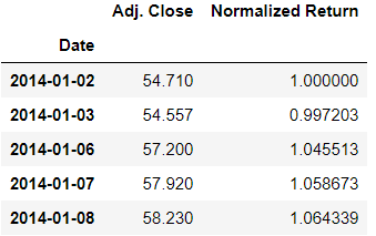
>>> aapl = quandl.get('WIKI/AAPL.11',start_date=start, end_date=end)>>> fb.head()

>>> twtr.head()
>>> aapl.head()
→ Finding returns
So first the normalized return will be calculated which is the value of adjusted close for each index divided by the initial value of adjusted close value.
>>> for s_df in (fb,twtr,aapl):
        s_df['Normalized Return'] = s_df['Adj. Close']/s_df.iloc[0]['Adj. Close']>>> fb.head()
→ Allocations
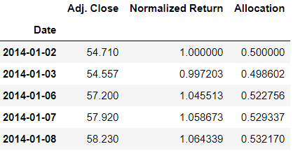
Now let’s assume the allocations for the three stocks. 50% of the money is allocated to Facebook stock, 30% of the money is allocated to Twitter stock and 20% of the money is allocated to Apple stock. So now the allocations are found out by multiplying the percent with the returns.
>>> for s_df, allocation in zip((fb,twtr,aapl),[0.5,0.3,0.2]):
        s_df['Allocation'] = s_df['Normalized Return']*allocation>>> fb.head()
→ Position value
Assuming that 1 lakh rupees is invested. So according to this the position value will be calculated which is the multiplication of the allocation and the investment.
>>> investment = 100000>>> for s_df in (fb,twtr,aapl):
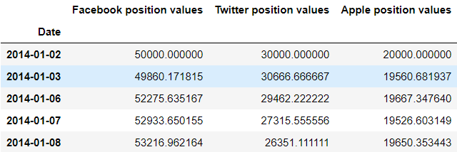
s_df['Position value'] = s_df['Allocation'] * investment>>> fb.head()
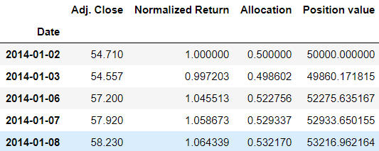
So the insight that can be drawn is that on 2nd January 2014 50000/- was allocated to Facebook and then on the next day since the stock went down the money became approximately 49860/- and on the third day, it again rose to approximately 52275/-. And so on, as the days change the value of the money keeps rising and falling accordingly.
Now let’s look into the position values for all the stocks.
>>> position_values = pd.concat([fb['Position value'],
>>> twtr['Position value'],aapl['Position value']],axis=1)>>> position_values.head()
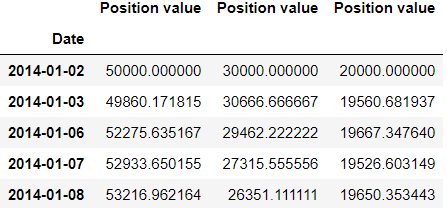
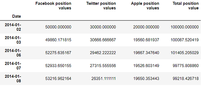
>>> position_values.columns = ['Facebook position values','Twitter position values', 'Apple position values']>>> position_values.head()
The total position can now be calculated by summing the values of all stocks position values.
>>> position_values['Total position value'] = position_values.sum(axis=1)>>> position_values.head()
>>> position_values.tail()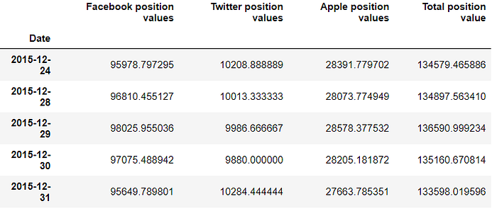
So as seen from the values above, investing in Facebook and apple would prove to be beneficial as the investment gives more return. But investing in Twitter is a loss.
→ Plotting
So keeping in mind that the initial investment of 1 lakh rupees, by plotting we can visualize if the money has increased or decreased by the end of the term and its trend.
>>> position_values['Total position value'].plot(figsize=(10,8))
>>> plt.title('Total portfolio value')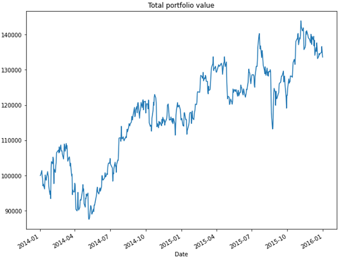
So by the end of the term, the value of money is at approximately 13 lakhs.
The stock position values can be plotted individually too to understand how the stocks grew.
>>> position_values.drop('Total position value',axis=1).plot(figsize=(10,8))
So the stock of Facebook has grown in an upward trend whereas the other two stocks didn't have much variance. In fact, Twitter had a downward trend.
→ Portfolio statistics
Various statistics like daily returns, average daily returns and standard deviation can be calculated. These statistics can help determine the Sharpe ratio too.
>>> position_values.head()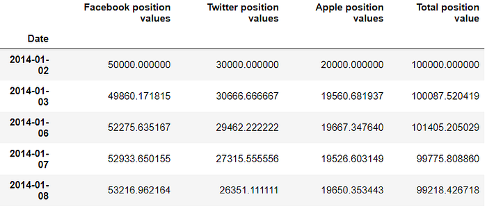
To calculate the daily return the pandas function ‘pct_change’ will be used. It calculates the percentage change between the current and a prior element. The periods to shift is 1.
>>> position_values['Daily return'] = position_values['Total position value'].pct_change(1)
>>> position_values.head()
The average daily return can be found by calling the mean() function on the daily returns.
>>> position_values['Daily return'].mean()
0.0007122766289206966
The standard deviation can be calculated by calling the ‘std()’ function on daily returns.
>>> position_values['Daily return'].std()
0.01651000095519752
→ Sharpe ratio
The Sharpe ratio is the average return received wrt the risk-free rate per unit of volatility. Volatility is the fluctuations in the price of a portfolio. The Sharpe ratio helps determine the return on investment when compared to its risk.
The greater the value of the Sharpe ratio, the more attractive the risk-adjusted return. The formula for the Sharpe ratio is:
where:
Rp=return of the portfolio
Rf=risk-free rate
σp=standard deviation of the portfolio’s excess return
The risk-free rate per unit is considered to be 0 here.
>>> sharpe_r = position_values['Daily return'].mean()/position_values['Daily return'].std()
>>> sharpe_r
0.04314213129687704
The annual Sharpe ratio can be calculated by multiplying ‘k’ value with the Sharpe ratio. The ‘k’ value is the root of the number of business days. There are 252 days where trade business is carried out and therefore k=252.
>>> annual_sharpe_r = sharpe_r * (252**0.5)
>>> annual_sharpe_r
0.6848601026449987
A Sharpe ratio greater than 1 is generally accepted to be a good value. A ratio higher than 2 is great and higher than 3 is excellent.