A Comprehensive Guide To Using Pandas For Data Science

A detailed guide with code to understand and practically implement Pandas when dealing with data.

What is Pandas?

Pandas is an open-source library that is used for data processing tasks like cleaning and preparation. It paves way for fast analysis of data and also has techniques for visualizing the data. It is built on top of the NumPy library.

To know more about the NumPy library, check my article here.

How to install Pandas?

1. Through command line using pip

pip install pandas

2. Through command line using Anaconda

conda install pandas

What is the series datatype of Pandas?

Series is in resemblance to a NumPy array but the difference is that series can be accessed by labels or it can be indexed by labels. Also, it can store any object type.

→ Importing libraries

>>> import numpy as np
>>> import pandas as pd

→ Creating series from various object types — list, array, dictionary

>>> headings = ['a', 'b', 'c']
>>> list1 = [11,22,33]
>>> arr1 = np.array(list1)
>>> dict1 = {'a':11, 'b':22, 'c':33}
>>> headings
['a', 'b', 'c']
>>> list1
[11, 22, 33]
>>> arr1
array([11, 22, 33])
>>> dict1
{'a': 11, 'b': 22, 'c': 33}

→ Passing the data argument when creating a series

>>> pd.Series(data = list1)
0    11
1    22
2    33
dtype: int64
>>> pd.Series(arr1)
0    11
1    22
2    33
dtype: int32
>>> pd.Series(dict1)
a    11
b    22
c    33
dtype: int64
>>> pd.Series(headings)
0    a
1    b
2    c
dtype: object

→ Passing the index values for customizing.

>>> pd.Series(data = list1, index = headings)
a    11
b    22
c    33
dtype: int64

→ Obtaining information from the series.

>>> series1 = pd.Series(dict1)
>>> series1
a    11
b    22
c    33
dtype: int64
>>> series1['a']
11

→ Operations on series

>>> dict2 = {'a':1, 'b':2, 'd':3}
>>> series2 = pd.Series(dict2)
>>> series2
a    1
b    2
d    3
dtype: int64
>>> series1
a    11
b    22
c    33
dtype: int64

Where there is a match, the operation is performed. When no match, a null value is returned.

>>> series1 + series2
a    12.0
b    24.0
c     NaN
d     NaN
dtype: float64

What are DataFrames in Pandas?

→ Creating dataframe

>>> from numpy.random import randn

The arguments passed are the values of the dataframe, the labels of the row and column. An important thing to note is that dataframes are built upon series. Below the columns, ‘y’ and ‘z’ are series only that share the common index. And the rows are also series.

>>> dataframe = pd.DataFrame(randn(3,2), ['a','b','c'], ['y', 'z'])
>>> dataframe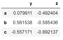

>>> type(dataframe)
pandas.core.frame.DataFrame

→ Obtaining information from the columns of dataframes using brackets and the SQL dot notation.

>>> dataframe['z']
a   -0.492404
b   -0.585436
c   -0.892137
Name: z, dtype: float64
>>> type(dataframe['z'])
pandas.core.series.Series
>>> dataframe.z
a   -0.492404
b   -0.585436
c   -0.892137
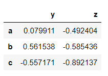
Name: z, dtype: float64
>>> dataframe[['y','z']]

→ Creating a new column.

>>> dataframe['new_col'] = dataframe['y'] - dataframe['z']
>>> dataframe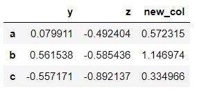

→ Dropping columns.

The axis has is an argument of the drop method which is zero by default. To drop a column, the axis value should be 1.

>>> dataframe.drop('new_col', axis = 1)

But this drop method is not inplace. That means the drop is not permanent. If the dataframe is printed again then the dropped column will be seen.

>>> dataframe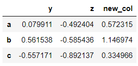

To make it occur inplace, we mention the inplace argument as true.

>>> dataframe.drop('new_col', axis = 1, inplace = True)
>>> dataframe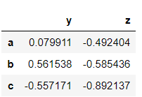

→ Dropping rows.

>>> dataframe.drop('c')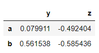

→ Obtaining information from rows of the dataframe using loc and iloc.

loc is the location and it obtains information of the row when the row name is passed. iloc is an index-based location wherein the index of the row is passed. For example, here row ‘c’ has an index value 2.

>>> dataframe.loc['c']
y   -0.557171
z   -0.892137
Name: c, dtype: float64
>>> type(dataframe.loc['c'])
pandas.core.series.Series
>>> dataframe.iloc[2]
y   -0.557171
z   -0.892137
Name: c, dtype: float64

→ Obtaining information with a combination of rows and columns.

>>> dataframe.loc['a','z']
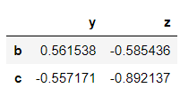
-0.4924042937068482
>>> dataframe.loc[['b','c'],['y','z']]

→ Obtaining information based on conditions.

>>> bool_df = dataframe > 0
>>> bool_df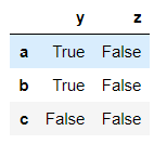

Shows null value where ever the condition is false.

>>> dataframe[bool_df]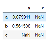

>>> dataframe[dataframe<0]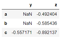

>>> dataframe['y'] > 0
a     True
b     True
c    False
Name: y, dtype: bool

Note that while grabbing rows, the null values are not shown. Since the values which satisfy the condition are only obtained.

>>> dataframe[dataframe['y']>0]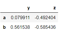

>>> dataframe[dataframe['z']<0]['y']
a    0.079911
b    0.561538
c   -0.557171
Name: y, dtype: float64

Applying multiple conditions. Make sure that you use ‘&’ instead of ‘and’ and ‘|’ instead of ‘or’. This is because the conditions compared are in the boolean form. ‘and’ and ‘or’ work only on single boolean values and not on series of boolean values.

>>> dataframe[(dataframe['y']>0) & (dataframe['z']<0)]

→ Dealing with indexes.

To reset the indexes or the row label, do the following. Again this does not occur inplace, so it has to be mentioned in the arguments.

>>> dataframe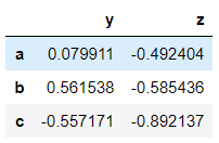

>>> dataframe.reset_index()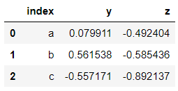

To set the index, we can create a new column and add it to the dataframe and then set it. Again the set index method is not inplace. It has to be mentioned explicitly.

>>> new_index = 'aa bb cc'.split()
>>> new_index
['aa', 'bb', 'cc']
>>> dataframe['new_col'] = new_index
>>> dataframe

>>> dataframe.set_index('new_col')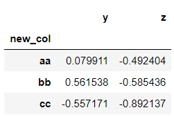

→ Dealing with multi-level index.

We start off by creating the index levels by forming two lists, then zipping it into a tuple and then calling the pandas method which creates the multi-index.

>>> list1 = ['a', 'a', 'a', 'b', 'b', 'b']
>>> list2 = [11,22,33,11,22,33]
>>> index_level = list(zip(list1,list2))
>>> index_level
[('a', 11), ('a', 22), ('a', 33), ('b', 11), ('b', 22), ('b', 33)]
>>> index_level = pd.MultiIndex.from_tuples(index_level)
>>> index_level
MultiIndex([('a', 11),
            ('a', 22),
            ('a', 33),
            ('b', 11),
            ('b', 22),
            ('b', 33)],
           )

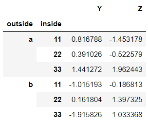
So as you can see, there is index ‘a’ and ‘b’ which has subparts 11,22,33 and inside it are the values. This is the index hierarchy.

>>> dataframe2 = pd.DataFrame(randn(6,2), index_level, ['Y','Z'])
>>> dataframe2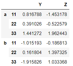

>>> dataframe2.loc['a']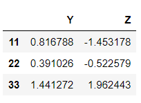

>>> dataframe2.loc['a'].loc[22]
Y    0.391026
Z   -0.522579
Name: 22, dtype: float64

Naming the indexes.

>>> dataframe2.index.names
FrozenList([None, None])
>>> dataframe2.index.names = ['outside', 'inside']
dataframe2

Obtaining the cross-section in a multi-level indexed dataframe. When the index ‘a’ is called, it only results in displaying the part of ‘a’.

>>> dataframe2.xs('a')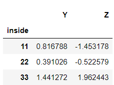

In case you want the subpart ‘22’ of both indexes ‘a’ and ‘b’, you do the following.

>>> dataframe2.xs(22, level = 'inside')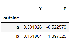

How to deal with missing data using Pandas?

If in the dataset there is a missing value then when using Pandas, it automatically denotes the missing value with a null value also denoted by NaN. So it is important to drop the missing values or fill the missing values so as to work on the data efficiently.

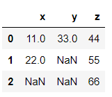
To denote null values, use np.nan.

>>> dataframe3 = {'x':[11,22,np.nan], 'y':[33, np.nan,np.nan], 'z':[44,55,66]}
>>> df = pd.DataFrame(dataframe3)
df

→ Dropping NaN values.

Now let’s drop the missing values from the dataframe. It drops the rows with missing values since the default argument axis= 0.

>>> df.dropna()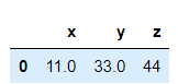

If you want to drop columns where there are null values, mention axis = 1.

>>> df.dropna(axis=1)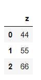

There is another argument called thresh which takes in an integer value. The integer value denotes the threshold for how many minimum non-Nan values should be present. So as you can see, the second row is retained since it has 2 non-Nan values when 2 is given as the value of thresh.

>>> df.dropna(thresh=2)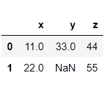

→ Filling NaN values.

>>> df.fillna(value='A values if filled')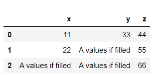

Usually, the mean is filled in place of NaN values.

>>> df['x'].fillna(value=df['x'].mean())
0    11.0
1    22.0
2    16.5
Name: x, dtype: float64

How to group data using Pandas?

At times, you are supposed to group rows together on the basis of the column and then perform some function of aggregation on it. GroupBy allows you to form these groups.

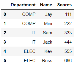
Creating a dataframe for grouping.

>>> data = {'Department':['COMP', 'COMP', 'IT', 'IT', 'ELEC', 'ELEC'],'Name':['Jay', 'Mini', 'Sam', 'Jack', 'Kev', 'Russ'],'Scores':[111,222,333,444,555,666]}
>>> dataframe4 = pd.DataFrame(data)
>>> dataframe4

Grouping by the department name.

>>> dataframe4.groupby('Department'
<pandas.core.groupby.generic.DataFrameGroupBy object at 0x000001A41A043AC8>

It returns the address. So to view it, store it in a variable.

>>> Dept = dataframe4.groupby('Department')

Now performing some functions, like getting the mean score or sum according to the department groups. Pandas automatically consider the numeric column since operations cannot be performed on strings.

>>> Dept.mean()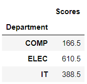

>>> Dept.sum()

>>> Dept.std()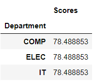

>>> Dept.std().loc['IT']
Scores    78.488853
Name: IT, dtype: float64

For counting the number of instances.

>>> Dept.count()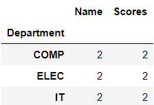

>>> Dept.max()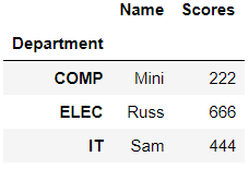

>>> Dept.describe()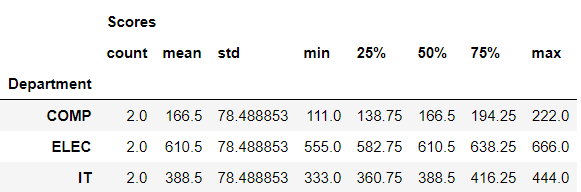

How to combine dataframes using Pandas?

→ Using concatenation.

It takes the dataframes and glues or sticks them together. It is important that the dimension matches along the axis while concatenating.

Creating dataframes.

>>> df1 = pd.DataFrame({'A':['a0','a1','a2','a3'], 'B':['b0','b1','b2','b3'],'C':['c0','c1','c2','c3'], 'D':['d0','d1','d2','d3']},index=[0,1,2,3])
>>> df1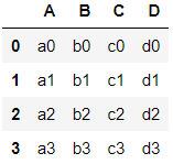

>>> df2 = pd.DataFrame({'A':['a4','a5','a6','a7'], 'B':['b4','b5','b6','b7'],'C':['c4','c5','c6','c7'], 'D':['d4','d5','d6','d7']},index=[4,5,6,7])
>>> df2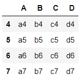

>>> pd.concat([df1,df2])

When concatenating along columns, use axis = 1. ‘Nan’ is filled where the data is missing.

>>> pd.concat([df1,df2], axis=1)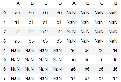

→ Using merge.

Just like the merge function of SQL tables, this merge function also allows dataframes to be merged.

Creating dataframes where there is one column common.

>>> df4 = pd.DataFrame({'value':['v0','v1','v2','v3'],'a':['a0','a1','a2','a3'],'b':['b0','b1','b2','b3']})
>>> df4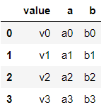

df5 = pd.DataFrame({'value':['v0','v1','v2','v3'],'c':['c0','c1','c2','c3'],'d':['d0','d1','d2','d3']})
>>> df5

>>> pd.merge(df4,df5,how='inner',on='value')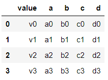

It performs an inner join on the common column ‘value’. The inner join is the default join. The other joins are outer join, right join and left join.

→ Using joining.

When there are dataframes with columns of different indexes then they can be merged into a single dataframe using join.

>>> df6 = pd.DataFrame({'a':['a0','a1','a2'],'b':['b0','b1','b2']},index=[0,1,2])
>>> df6

>>> df7 = pd.DataFrame({'c':['c0','c2','c3'],'d':['d0','d2','d3']},
index=[0,2,3])
>>> df7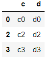

>>> df6.join(df7)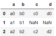

>>> df7.join(df6)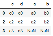

What different operations can be performed on Pandas dataframe?

>>> df8 = pd.DataFrame({'a':[11,22,33,22],'b':[1,2,3,4],'c':['aa','bb','cc','dd']})
>>> df8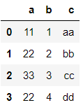

→ Getting unique values and the number of unique values.

>>> df8['a'].unique()
array([11, 22, 33], dtype=int64)
>>> df8['a'].nunique()
3
>>> df8['a'].value_counts()
22    2
11    1
33    1
Name: a, dtype: int64

→ Applying inbuilt and custom functions to a dataframe.

>>> def func(x):
       return x+x
>>> df8['b'].apply(func)
0    2
1    4
2    6
3    8
Name: b, dtype: int64
>>> df8['c'].apply(len)
0    2
1    2
2    2
3    2
Name: c, dtype: int64
>>> df8['a'].apply(lambda x: x*x)
0     121
1     484
2    1089
3     484
Name: a, dtype: int64

→ To get column names and information about the index.

>>> df8.columns
Index(['a', 'b', 'c'], dtype='object')
>>> df8.index
RangeIndex(start=0, stop=4, step=1)

→ Sorting according to a column.

>>> df8.sort_values('a')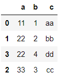

→ Finding null values.

>>> df8.isnull()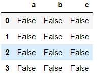

>>> df8.isnull().sum()
a    0
b    0
c    0
dtype: int64

→ Creating a pivot table.

Method pivot_table() takes 3 main arguments: values, index, columns.

>>> df9 = pd.DataFrame({'a':['jam','jam','jam','milk','milk','milk'],'b':['red','red','white','white','red','red'],'c':['yes','no','yes','no','yes','no'],'d':[11,33,22,55,44,11]})
>>> df9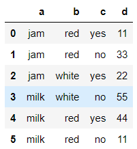

>>> df9.pivot_table(values='d', index=['a','b'], columns='c')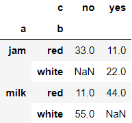

How to read and write data for different file formats using Pandas?

The different formats can be CSV, HTML, SQL and Excel. To work with SQL databases, an additional library has to be installed as follows:

pip/conda install sqlalchemy

→ Dealing with CSV files.

First reading the file, then displaying the dataframe followed by writing to the file.

>>> df10 = pd.read_csv('data.csv')
>>> df10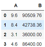

>>> df10.to_csv('data_output')
>>> pd.read_csv('data_output')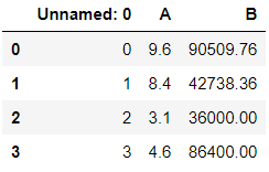

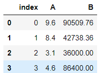
To avoid this unnamed index to form, set the argument index to false.

>>> df10.to_csv('data_output',index=False)
>>> pd.read_csv('data_output')

→ Dealing with Excel files.

>>> df11 = pd.read_excel('dataset.xlsx')
>>> df11

>>> df11.to_excel('dataset_output.xlsx',sheet_name='dataset sheet')

→ Dealing with HTML input.

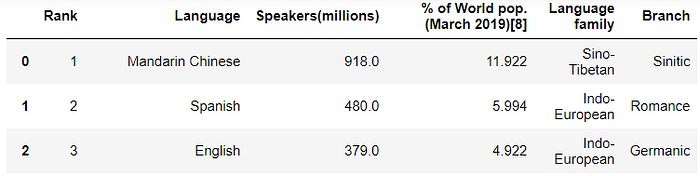
Choose a website that has a table. Using Pandas the webpage will be read in the form of a list.

>>> data = pd.read_html('https://en.wikipedia.org/wiki/List_of_languages_by_number_of_native_speakers')
>>> type(data)
list
>>> data[0]

→ Dealing with SQL database.

Remember that every SQL engine has a different way of dealing with it. Here a simple SQL database is made stored in the memory and Pandas will be used. The engine is created where the database is stored in memory. Then later a dataframe is written to SQL giving it a name and the engine. Then the SQL dataframe is read.

>>> from sqlalchemy import create_engine
>>> sql_engine = create_engine('sqlite:///:memory:')
>>> df10.to_sql('sql_data',sql_engine)
>>> sql_df = pd.read_sql('sql_data',sql_engine)
>>> sql_df

For more detailed information on Pandas, check the official documentation here.

Refer to the notebook for code here.

Books to refer to:

Hands-on Data Analysis and Visualization with Pandas

Python Data Analytics: The Ultimate Guide To Get Started With Data Analysis Using Python, NumPy and…

Python for Data Analysis, 2e: Data Wrangling with Pandas, Numpy, and Ipython

Python Data Analytics: With Pandas, NumPy, and Matplotlib

Reach out to me: LinkedIn

Check out my other work: GitHub